Software requirements
We advise the following software suites:
A current PostgreSQL database with PostGIS and MobilityDB is first required. I recommend using the latest releases available for your OS of choice, even though MobilityDB works with older releases of PostgreSQL and PostGIS, too. If you’d rather not create MobilityDB from scratch, you can also use a Docker container from https://registry.hub.docker.com/r/codewit/mobilitydb.
The second thing you’ll need is a tool to transfer our raw flight data, which is provided as sizable csv files, to our database. I typically use ogr2ogr, a command-line tool included with Gdal, for this kind of task.
Finally, we’ll use “Quantum GIS,” a feature-rich GIS-client that is available for different operating systems, to graphically represent our results.
Here is a brief description of my setup:
- Ubuntu (20.04.3),
- PostgreSQL (13),
- PostGIS (3.2.1),
- MobilityDB (1.0.0),
- ogr2ogr (3.0.4),
- QGIS (3.20.3)
Data allocation and preparation
Our analysis is based on OpenSky Network data about past flights that can be used for non-commercial purposes. OpenSky gave snapshots of the full state vector data as of Monday for the last six months. Time (updated every second), ICAO24, lat/lon, speed, heading, vertrate, callsign, onground, alert/spi, squawk, baro/geoaltitude, lastposupdate, and lastcontact are all part of these data sets. You can find a thorough description here.
Let’s get to the analysis by downloading historical datasets now that the theory is finished. This post is based on 24 CSV files with flight information for February 28, 2012. You can download them from this page.
Next, we’ll create a brand-new PostgreSQL database with PostGIS and MobilityDB extensions enabled. Our state vectors will be kept in the database.
postgres=# create database flightanalysis; CREATE DATABASE postgres=# \c flightanalysis You are now connected to database "flightanalysis" as user "postgres." flightanalysis=# create extension MobilityDB cascade; NOTICE: installing required extension "postgis" CREATE EXTENSION flightanalysis=# \dx List of installed extensions Name, Version, Schema, and Description ------------+---------+------------+------------------------------------------------------------ mobilitydb | 1.0.0 | public | MobilityDB Extension plpgsql | 1.0 | pg_catalog | PL/pgSQL procedural language postgis | 3.2.1 | public | PostGIS geometry and geography spatial types and functions (3 rows)
OpenSky’s dataset descriptions give us a data structure for a staging table that keeps raw state vectors that haven’t been changed.
create table tvectors ( ogc_fid integer default nextval('flightsegments_ogc_fid_seq'::regclass) not null constraint flightsegments_pkey primary key, time integer, ftime timestamp with time zone, icao24 varchar, lat double precision, lon double precision, velocity double precision, heading double precision, vertrate double precision, callsign varchar, onground boolean, alert boolean, spi boolean, squawk integer, baroaltitude double precision, geoaltitude double precision, lastposupdate double precision, lastcontact double precision ); create index idx_points_icao24 on tvectors (icao24, callsign);
Now, we can import state vectors into our database for flight analysis from a directory with uncompressed csv files as follows:
for f in `ls *.csv`; do ogr2ogr -f PostgreSQL PG: "user=postgres, dbname=flightanalysis" $f -oo AUTODETECT_TYPE=YES -nln tvectors --config PG_USE_COPY YES done
How many imported vectors were there?
flightanalysis=# select count(*) from tvectors; count ---------- 52261548 (1 row)
Now, in order to use MobilityDB to analyze our vectors, we need to turn our native position data into trajectories.
MobilityDB offers various data types to model trajectories, such as tgeompoint, which represents a temporal geometry point type.
create table if not exists flightsegments ( icao24 varchar not null, callsign varchar not null, trip tgeompoint, traj geometry(Geometry,4326), constraint flightsegment_2_pkey primary key (icao24, callsign) ); create index idx_trip on flightsegments using gist (trip); create index idx_traj on flightsegments using gist (traj);
Trajectories must be generated by choosing vectors by ICAO-24 and callsigns ordered by time in order to track individual flights from aircraft.
In our staging table, timestamps (column time) are initially displayed as unix timestamps. We’ll convert unix timestamps to timestamps with time zones first for convenience.
update tvectors set ftime= to_timestamp(time) AT TIME ZONE 'UTC'; create index idx_points_ftime on tvectors (ftime);
We can finally create our trajectories by combining locations by ICAO-24 and callsigns ordered by time.
insert (ICAO 24, callsign, trip) into the flight segments SELECT icao24, callsign, tgeompoint_seq(array_agg(tgeompoint_inst(ST_SetSRID(ST_MakePoint(Lon, Lat), 4326), ftime) ORDER BY ftime)) from tvectors where lon is not null and lat is not null group by icao24, callsign;
To visualize our aggregated vectors in QGIS, someone must extract the vectors’ raw geometries from tgeompoint, as this data type is not supported natively out of the box from QGIS.
To create a geometrically simplified version for better performance, we’ll utilize st_simplify on top of the trajectory. It’s important to note that there are also simplification methods in MobilityDB that make the whole trajectory easier to understand, not just its geometry.
update flightsegments set traj = st_simplify(trajectory(trip)::geometry, 0.001)::geometry;
You can see how many vectors there are in these freely downloadable datasets for just one single day from the images below.
The data needs to be further cleaned and filtered because it is noisy, as you can see in the image. Defective and misleading results result from coverage and recording gaps that produce global trajectories. But we’ll skip this complicated cleaning process today (we might talk about it in a later blog post) and instead focus on a small part of our analysis.
Analysis
Investigating the trajectories and running some intriguing scenarios will be helpful.
Amount of unique airframes (as determined by icao24)
flightanalysis = # select count(distinct icao24) from flightsegments; count --------- 41663 (1 row)
Average flight duration
flightanalysis=# select st_length(trajectory(trip::tgeogpoint)) > 0; avg(duration(trip)) from flightsegments ----------------- 03:50:48.245525 (1 row)
Between [2022-02-28 00:00:00+00 and 2022-02-28 03:00:00+00] flight vectors will intersect Iceland.
Download and import country borders from Natural Earth first in order to perform this type of analysis.
select icao24, callsign, trajectory(atPeriod(T.Trip, '[2022-02-28 00:00:00+00, [2022-2-28 03:00:00+00]'::period)) FROM flightsegments T, ne_10m_admin_0_countries R WHERE T.Trip && stbox(R.geom, '[2022-02-28 00:00:00+00, [2022-02-28 03:00:00+00]'::period) AND st_intersects(trajectory(atPeriod(T.Trip, '[2022-02-28 00:00:00+00, [2022-2-28 03:00:00+00]'::period)), r.geom) and R.name = 'Iceland' and st_length(trajectory(atPeriod(T.Trip, '[2022-02-28 00:00:00+00, [2022-2-28 03:00:00+00]'::period))::geography) > 0
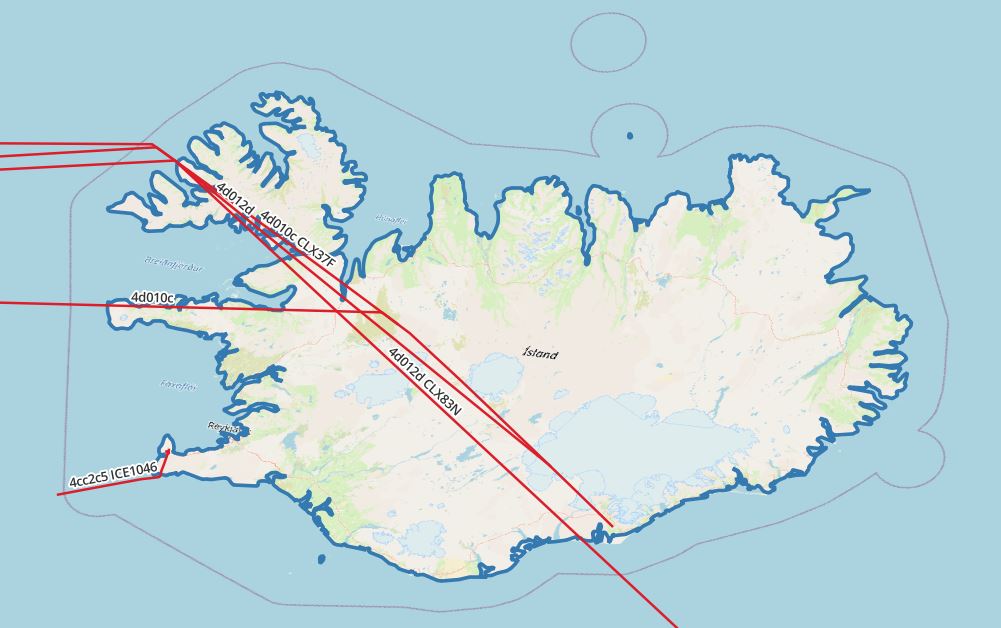
Figure 1: Vectors intersecting with Iceland
Flight vectors intersecting Iceland for the duration of the flyover between [2022-02-28 00:00:00+00, 2022-02-28 03:00:00+00]
select icao24, callsign, (duration( (atgeometry((atPeriod(T.Trip::tgeompoint, '[2022-02-28 00:00:00+00, [2022-02-28 03:00:00+00]'::period)), R.geom))))::varchar, trajectory( atgeometry((atPeriod(T.Trip::tgeompoint, '[2022-02-28 00:00:00+00, [2022-02-28 03:00:00+00]'::period)), R.geom)) FROM flightsegments T, ne_10m_admin_0_countries R WHERE T.Trip && stbox(R.geom, '[2022-02-28 00:00:00+00, [2022-02-28 03:00:00+00]'::period) AND st_intersects(trajectory(atPeriod(T.Trip, '[2022-02-28 00:00:00+00, [2022-2-28 03:00:00+00]'::period)), r.geom) and R.name = 'Iceland' and st_length(trajectory(atPeriod(T.Trip, '[2022-02-28 00:00:00+00, [2022-2-28 03:00:00+00]'::period))::geography) > 0
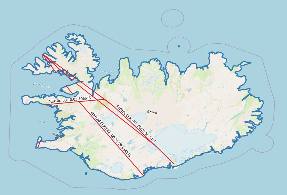
Figure 2: Clipped vectors intersecting with Iceland
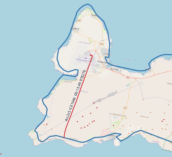
Figure 3 shows a clipped vector intersecting with Iceland and the callsign “ICE1046” for ICAO24.
When Iceland is crossed between [2022-02-28 00:00:00+00] and [2022-02-28 03:00:00+00], the border for each individual airframe and callsign is crossed.
Take note that during this flight, the plane did not leave the country.
with segments as ( select icao24, callsign, unnest(sequences( atgeometry( (atPeriod(T.Trip::tgeompoint, '[2022-02-28 00:00:00+00, [2022-02-28 03:00:00+00]'::period)), R.geom))) segment FROM flightsegments T, ne_10m_admin_0_countries R WHERE T.Trip && stbox(R.geom, '[2022-02-28 00:00:00+00, [2022-02-28 03:00:00+00]'::period) AND st_intersects(trajectory(atPeriod(T.Trip, '[2022-02-28 00:00:00+00, [2022-2-28 03:00:00+00]'::period)), r.geom) and R.name = 'Iceland' and trim(callsign) = 'ICE1046' and st_length(trajectory(atPeriod(T.Trip, '[2022-02-28 00:00:00+00, [2022-2-28 03:00:00+00]'::period))::geography) > 0) select icao24, callsign, st_startpoint(getvalues(segment)), st_endpoint(getvalues(segment)), starttimestamp(segment), endtimestamp(segment) from segments
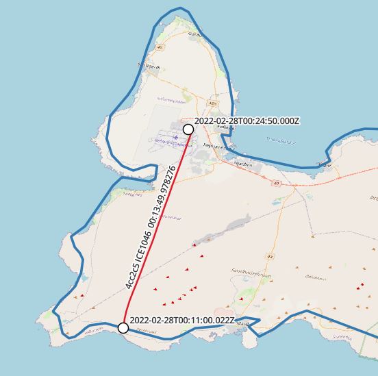
Figure 4: Border crossing, icao24 “4cc2c5” callsign “ICE1046”
Outlook
The study of spatio-temporal data is significantly made easier by MobilityDB’s comprehensive feature stack. If I’m permitted to think of any other applications for it, I can think of a number of businesses where it could be used in a clever and effective way. Toll collection systems, security, and logistics are a few examples. Finally, its future version will open the door for new applications ranging from production scenarios to research and test usage.
About Enteros
Enteros offers a patented database performance management SaaS platform. It proactively identifies root causes of complex business-impacting database scalability and performance issues across a growing number of clouds, RDBMS, NoSQL, and machine learning database platforms.
The views expressed on this blog are those of the author and do not necessarily reflect the opinions of Enteros Inc. This blog may contain links to the content of third-party sites. By providing such links, Enteros Inc. does not adopt, guarantee, approve, or endorse the information, views, or products available on such sites.
Are you interested in writing for Enteros’ Blog? Please send us a pitch!
RELATED POSTS
How Predictive SQL Performance Analytics Accelerates Application Modernization
- 18 June 2026
- Database Performance Management
Application modernization has become a strategic priority for enterprises seeking greater agility, scalability, and competitive advantage. Organizations are increasingly transforming legacy systems into cloud-ready, data-driven, and highly scalable architectures to meet growing digital demands. Whether migrating monolithic applications to microservices, adopting cloud-native platforms, or modernizing data infrastructure, enterprises face a common challenge: maintaining database performance … Continue reading “How Predictive SQL Performance Analytics Accelerates Application Modernization”
How to Modernize BFSI Cost Management with Enteros Database Software and Cost Attribution Analytics
Introduction The Banking, Financial Services, and Insurance (BFSI) industry is undergoing rapid transformation driven by digital banking, fintech innovation, regulatory requirements, customer expectations, and growing data volumes. As organizations continue investing in cloud platforms, digital services, AI-powered applications, and advanced analytics, technology spending has become one of the largest operational expenses across the financial sector. … Continue reading “How to Modernize BFSI Cost Management with Enteros Database Software and Cost Attribution Analytics”
The Business Value of AI-Powered Database Performance Analytics for Digital Enterprises
In today’s digital economy, enterprise success increasingly depends on application performance, operational agility, and the ability to deliver seamless user experiences at scale. From e-commerce platforms and financial services to SaaS applications and digital healthcare systems, businesses rely heavily on data-driven applications to serve customers, process transactions, and generate insights in real time. At the … Continue reading “The Business Value of AI-Powered Database Performance Analytics for Digital Enterprises”
How to Transform Financial Operations with Enteros Database Software and Growth Intelligence
- 17 June 2026
- Database Performance Management
Introduction Financial institutions operate in one of the most data-intensive and highly regulated environments in the world. Banks, insurance companies, investment firms, fintech organizations, and financial service providers rely heavily on digital platforms to process transactions, manage risk, deliver customer experiences, and drive business growth. Today’s financial ecosystems support: Digital banking platforms Payment processing systems … Continue reading “How to Transform Financial Operations with Enteros Database Software and Growth Intelligence”