Scaling and Full Parallelism Experimentation in PostgreSQL

Preamble

PostgreSQL’s ability to scale to many cores and, subsequently, to many machines has been discussed extensively. For a very long time, running PostgreSQL on a server farm was not an option. This has unquestionably changed, though. Scaling PostgreSQL and executing a single query across multiple CPUs are two areas that have seen a lot of development. The first version of PostgreSQL that allowed running a query across multiple nodes was 9.6. PostgreSQL is getting better all the time thanks to continued development.

Scaling PostgreSQL to “1 billion rows / second”

Even though the idea that PostgreSQL can grow indefinitely is not new, it is still exciting to keep pushing the limits of this popular open-source database.

Scaling with parallel queries

Traditionally, a query in PostgreSQL used only one CPU core. Of course, this used to be a serious restriction that has thankfully been lifted. PostgreSQL already supports doing a lot of things in parallel. As the project moves forward, it will be possible to do more things in parallel, and multicore systems will help with a larger number of queries.

We’ve made a simple data structure to show how parallel processing can help a simple query:

 node=# d t_demo Table "public.t_demo" Column |  Type   | Collation | Nullable |              Default --------+---------+-----------+----------+------------------------------------ id     | integer |           | not null | nextval('t_demo_id_seq'::regclass) grp    | integer |           |          | data   | real    |           |          | Indexes: "idx_id" btree (id)

This test’s query is attractive: It merely counts how many rows there are in each group.

 SELECT         grp, count(data) FROM            t_demo GROUP BY   1;

When running in parallel mode, our version of the optimizer can come up with the following best plan:

 node=# EXPLAIN SELECT grp, partial.count(data) FROM public.t_demo GROUP BY grp; QUERY PLAN -------------------------------------------------------------------------------------------------- Finalize GroupAggregate  (cost=635312.96..635314.26 rows=10 width=12) Group Key: grp -> Sort (cost (cost=635312.96..635313.36 rows = 160 width = 12) Sort Key: grp ->  Gather  (cost=635291.01..635307.10 rows=160 width=12) Workers Planned: 16 ->  Partial HashAggregate  (cost=634291.01..634291.10 rows=10 width=12) Group Key: grp ->  Parallel Seq Scan on t_demo  (cost=0.00..603041.01 rows=6250000 width=8)

PostgreSQL will use 16 worker processes to process the large table. If your system has at least 16 CPU cores, the performance will pretty much go up in a straight line as you add more worker processes. The data will be aggregated by each worker, and the partial aggregates will then be added. This linear trend is very important because it is needed to use hundreds or thousands of CPUs at the same time.

Because a single database node can add up millions of rows so quickly, a single box is usually enough for most applications. However, if data growth continues, scaling to an excessive number of nodes may be required.

Performance will increase based on the number of processes used, assuming our data node has 16 CPU cores (Google Cloud Box) and 100 million rows:

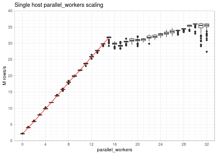
The fact that the line climbs straight to 16 cores is the first significant finding. It’s also intriguing to see that even if you use more than 16 processes to complete the task, you can still gain a little bit of speed. The advantage you can see here is due to Intel Hyperthreading; given this kind of query, you can anticipate a boost of about 15%. For a simple aggregation, you can process up to 40 million rows per second on a single database node (VM).

PostgreSQL parallel queries in a PostgreSQL server farm

Adding servers is the only way to achieve the desired goal of processing more than 1 billion rows per second.

The data will reside on the actual nodes and be stored in a distributed partitioned table.

In order to verify that we do, in fact, process twice as much data in the same amount of time, a second server is added in the first step.

This is the strategy to be used:

 EXPLAIN ANALYZE SELECT grp, COUNT(data) FROM t_demo group by 1; query plan ------------------------------------------------------------------------------------------------------------ Finalize HashAggregate  (cost=0.02..0.03 rows=1 width=12) (actual time=2706.764..2706.768 rows=10 loops=1) Group Key: t_demo.grp ->  Append  (cost=0.01..0.01 rows=1 width=0) (actual time=2486.349..2706.735 rows=20 loops=1) ->  Foreign Scan  (cost=0.00..0.00 rows=0 width=0) (actual time=0.818..0.822 rows=10 loops=1) ->  Foreign Scan  (cost=0.00..0.00 rows=0 width=0) (actual time=0.755..0.758 rows=10 loops=1) ->  Partial HashAggregate  (cost=0.01..0.01 rows=1 width=0) (never executed) Group Key: t_demo.grp -> Seq Scan on t_demo (cost = 0.00..0.00 rows = 1 width = 8) (never executed) Planning time: 0.200 ms Execution time: 2710.888 ms

The beauty of this example is that the execution time does not change even though 100 million rows have been deployed on each database server.

Now let’s run the same query on a table with 32 x 100 million rows:

 node=# EXPLAIN ANALYZE SELECT         grp, count(data) FROM            t_demo group by 1; query plan ------------------------------------------------------------------------------------------------------------ Finalize HashAggregate  (cost=0.02..0.03 rows=1 width=12) (actual time=2840.335..2840.340 rows=10 loops=1) Group Key: t_demo.grp ->  Append  (cost=0.01..0.01 rows=1 width=0) (actual time=2047.930..2840.015 rows=320 loops=1) ->  Foreign Scan  (cost=0.00..0.00 rows=0 width=0) (actual time=1.050..1.052 rows=10 loops=1) ->  Foreign Scan  (cost=0.00..0.00 rows=0 width=0) (actual time=1.000..1.002 rows=10 loops=1) ->  Foreign Scan  (cost=0.00..0.00 rows=0 width=0) (actual time=0.793..0.796 rows=10 loops=1) ->  Foreign Scan  (cost=0.00..0.00 rows=0 width=0) (actual time=0.776..0.779 rows=10 loops=1) ... ->  Foreign Scan  (cost=0.00..0.00 rows=0 width=0) (actual time=1.112..1.116 rows=10 loops=1) ->  Foreign Scan  (cost=0.00..0.00 rows=0 width=0) (actual time=1.537..1.541 rows=10 loops=1) -> Partial HashAggregate (cost = 0.01 to 0.01; rows = 1; width = 0) (never executed) Group Key: t_demo.grp -> Seq Scan on t_demo (cost = 0.00..0.00 rows = 1 width = 8) (never executed) Planning time: 0.955 ms Execution time: 2910.367 ms

Wow, 3.2 billion rows take less than 3 seconds to complete!

This is the end result:

 node=# SELECT grp, count(data) FROM t_demo GROUP BY 1; grp |   count -----+----------- 6 | 320000000 7 | 320000000 0 | 320000000 9 | 320000000 5 | 320000000 4 | 320000000 3 | 320000000 2 | 320000000 1 | 320000000 8 | 320000000 (10 rows)

There are 3.2 billion rows total on those shards.

The most important thing we learned is that shards can be added to this type of query as needed when performance needs or data volumes grow. With each additional node, PostgreSQL will scale nicely.

Implementing scalability

What is then actually required to get those outcomes? First off, PostgreSQL 9.6 vanilla does not support it. PostgreSQL 10.0 will have the feature that PostgreSQL FDW needs to push down aggregates to a remote host, so that was the first thing we needed. The simple thing is that. Teaching PostgreSQL that all shards must operate in parallel is the hardest part. Fortunately, there was a patch available that made it possible for “append” nodes to fetch data simultaneously. A crucial prerequisite for our code to function is parallel appending.

But there’s more: PostgreSQL previously could only aggregate data after it had been linked. In essence, this constraint has prevented many performance improvements. We were able to build on top of Kyotaro Horiguchi’s fantastic work to remove this restriction, which allowed us to aggregate a lot of data and actually reach 1 billion rows per second. Given how hard the assignment was, it is more than important to point out Kyotaro’s contributions. Without him, it is very unlikely that we would have been successful.

However, more is required to make this work: Postgres fdw is frequently used in our solution. Postgres fdw uses a cursor on the remote side to make it possible to get a lot of data. Cursors cannot yet be fully parallelized between PostgreSQL 9.6 and PostgreSQL 10.0 at this time. We had to get rid of this rule so that all CPU cores on the remote machines could be used at the same time.

To complete the map-reduce style aggregation in this case, a few (at the time) handwritten aggregates are required. That is easily accomplished because it only requires a short extension.

JIT compilation and other speedups

Even though being able to process 1 billion rows per second is impressive, PostgreSQL will have even more cool features in the future. As JIT compilation and other optimizations (like tuple deformation, column store, etc.) start to make their way into PostgreSQL, we will get the same results with fewer and fewer CPUs. In order to achieve the same performance, you can use fewer and smaller servers.

Since we didn’t use any of these optimizations in our test, we know there is still a lot of room for improvement. The key takeaway from this is that we were able to demonstrate PostgreSQL’s ability to scale to hundreds or even thousands of CPUs that can work together in a cluster to process the same query.

Improving PostgreSQL scalability even more

So far, only one “master” server and a few shards have been employed. This architecture is adequate in the majority of situations. However, keep in mind that it is also possible to arrange servers into a tree, which can be useful for some calculations that are even more complex.

About Enteros

​​​​Enteros offers a patented database performance management SaaS platform. It finds the root causes of complex database scalability and performance problems that affect business across a growing number of cloud, RDBMS, NoSQL, and machine learning database platforms.