Pandas instead of SQL: Working with data in a new way

Pandas instead of SQL: Working with data in a new way

​​

Previously, SQL as a tool was enough for research analysis: quick data search and preliminary report on data.

Nowadays, data come in different forms and do not always refer to them as “relational databases”. They can be CSV files, plain text, Parquet, HDF5, andmany others. This is where the Pandas library can help you.

What is Pandas?

Pandas is a data analysis and processing package written in Python. Its code is open-source, and Anaconda developers back it up. This library excels at working with structured (tabular) data. The documentation contains more information. Pandas allow you to create data queries, among other things.

A declarative language is SQL. It enables you to declare everything so that a query resembles a regular English sentence. Pandas have a syntax that is considerably different from SQL. You apply operations to a dataset for conversion and modification and link them together.

SQL parsing

A SQL query is made up of several keywords. Between these words, you’ll find more data properties that you’ll want to look at. Here’s an example of a query framework that doesn’t include any specifics:

SELECT... FROM... WHERE...
GROUP BY...
ORDER BY...
LIMIT... OFFSET...

Other expressions exist, but these are the most common. To use Pandas with words, you must first load the data:

import pandas as pd

airports = pd.read_csv('data/airports.csv')
airport_freq = pd.read_csv('data/airport-frequencies.csv')
runways = pd.read_csv('data/runways.csv')

You can download this data here.

SELECT, WHERE, DISTINCT, LIMIT

Several expressions with the SELECT operator are shown below. LIMIT is used to cut off unnecessary results, and WHERE filters them out. To eliminate duplicate results, use the DISTINCT function..

SELECT with multiple conditions

Several selection conditions are combined using the operand &. If you only want a subset of some columns from a table, this subset is used in another pair of square brackets.

ORDER BY

By default, Pandas will sort the data in ascending order. For reverse sorting use the expression ascending=False.

IN and NOT IN

To filter not a single value but whole lists, there is an IN condition. In Pandas, the .isin() operator works exactly the same way. To override any condition, use ~ (tilde).

GROUP BY, COUNT, ORDER BY

Grouping is performed using the .groupby() operator. There is a small difference between COUNT semantics in SQL and Pandas. In Pandas .count() will return non-null/NaN values. To get a result like in SQL, use .size().

Below is a grouping by several fields. By default, Pandas sorts by the same field list, so in the first example, there is no need for .sort_values(). If you want to use different fields for sorting or DESC instead of ASC as in the second example, you need to specify the selection explicitly:

The use of .to_frame() and .reset_index() is determined by sorting by a specific field (size). This field must be part of the DataFrame type. After grouping in Pandas, the result is another type called GroupByObject. Therefore you need to convert it back to DataFrame. With .reset_index(), the line numbering for the data frame is restarted.

HAVING

In SQL, you can additionally filter grouped data using the HAVING condition. In Pandas, you can use .filter() and provide the Python function (or lambda expression), which will return True if a group of data is to be included in the result.

The first N records

Let’s say some preliminary queries have been made and there is now a data frame named by_country that contains the number of airports in each country:

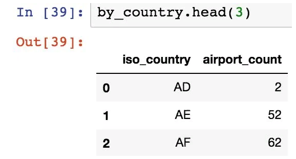
In the following example, let’s organize airport_count data and select only the first 10 countries with the largest number of airports. The second example is a more complex case, where we select the “next 10” after the first 10 entries:

Pandas instead of SQL: Working with data in a new way

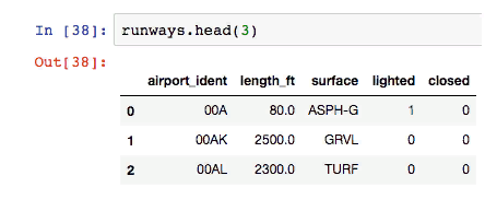
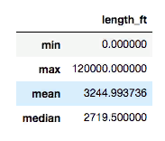
Considering the data frame above (runway data), let’s calculate the minimum, maximum, and average runway length.

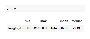
Note that with an SQL query, the data is a column. But in Pandas, the data is represented by rows.

The data frame can be easily transposed with .T to get the columns.

JOIN

Use .merge() to attach data frames to Pandas. You need to specify which columns to join (left_on and right_on) and the connection type: inner (default), left (corresponds to LEFT OUTER in SQL), right (RIGHT OUTER in SQL) or outer (FULL OUTER in SQL).

UNION ALL and UNION

pd.concat() is the UNION ALL equivalent in SQL.

The UNION equivalent (deduplication) is .drop_duplicates().

INSERT

So far, only sampling has been performed, but data can be changed during the preliminary analysis. In Pandas, there is no INSERT equivalent in SQL to add the required data. Instead, you should create a new data frame containing new records and then combine the two frames.

UPDATE

Suppose now you need to fix some incorrect data in the original frame.

DELETE

The easiest and most convenient way to remove data from a frame in Pandas is to split the frame into rows. Then get line indices and use them in the .drop() method.

Variability

By default, most operators in Pandas return a new object. Some operators accept inplace=True, which allows them to work with the original data frame instead of the new one. For example, you can reset the index in a place like this:

df.reset_index(drop=True, inplace=True)

However, the .loc operator (above in the example with UPDATE) simply finds the record indexes to update them, and the values change on the spot. Also, if all values in a column are updated (df[‘url’] = ‘http://google.com’) or a new column is added (df[‘total_cost’] = df[‘price’] * df[‘quantity’]), these data will change in place.

Pandas is more than just a query mechanism. Other transformations can be done with data.

Exporting to many formats

df.to_csv(...) # in csv file
df.to_hdf(...) # in an HDF5 file
df.to_pickle(...) # into the serialized object
df.to_sql(...) # to an SQL database
df.to_excel(...) # to an Excel file
df.to_json(...) # into JSON string
df.to_html(...) # display as an HTML table
df.to_feather(...) # in binary feather format
df.to_latex(...) # in a table environment
df.to_stata(...) # into Stata binary data files
df.to_msgpack(...) # msgpack-object (serialization)
df.to_gbq(...) # in the BigQuery-table (Google)
df.to_string(...) # into console output
df.to_clipboard(...) # in the clipboard that can be inserted into Excel

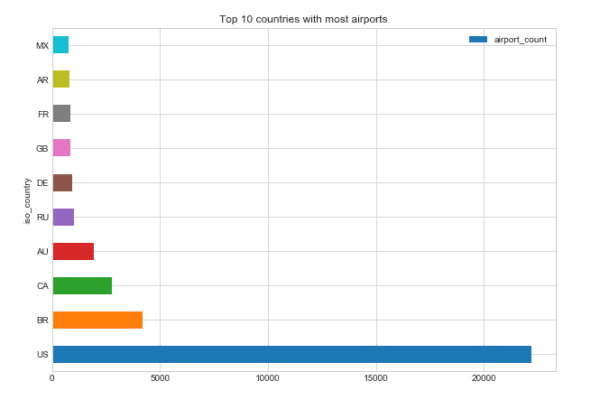
Drawing up charts

top_10.plot(
x='iso_country',
y='airport_count',
kind='barh',
figsize=(10, 7),
title='Top 10 countries with most airports')

We’ll get it:

Opportunity to share your work

The best place to publish Pandas queries, charts, and the like is the Jupyter notebook. Some people (like Jake Vanderplas) even publish whole books there. It is easy to create a new entry in the notebook:

$ pip install jupyter
$ jupyter notebook

After that you can:

• go to the address localhost:8888;
• press “New” and give your notebook a name;
• query and display the data;
• create a GitHub repository and add your notebook (a file with the extension .ipynb).

GitHub has an excellent built-in Jupyter notepad viewer with a Markdown design.

Why Combine Pandas and SQL

Enteros

About Enteros

IT organizations routinely spend days and weeks troubleshooting production database performance issues across multitudes of critical business systems. Fast and reliable resolution of database performance problems by Enteros enables businesses to generate and save millions of direct revenue, minimize waste of employees’ productivity, reduce the number of licenses, servers, and cloud resources and maximize the productivity of the application, database, and IT operations teams.